last update 06/17/2023
Release 3.5.3

BassCADe-Web-Help

Link to download page

Diese Hilfe in deutsch.

The content of this page is mostly common with the internal BassCADe BASSe.HLP file. Because the old (RTF based) Microsoft helpfile-format is not more installed per default of Windows installation. This additional page will provided as online version standard HTML.
As mentioned in the software: All content in this file is protected by copyright, all rights reserved. It is not allowed to copy or publish any content without permission of the author.

Overview:

  1. General
  2. Main window
  3. Speaker characteristics (TSP)
  4. Advice for a box type
  5. Open box
  6. Contained box
  7. Reflex box
  8. Contained band pass box
  9. Vented band pass box
  10. Comparision of simulations
  11. Exponential horn systems
  12. Transmission line (TML)
  13. Options and setup
  14. BassCADe configuration files
  15. Standing box housing
  16. Car-woofer housing
  17. Pyramide housing
  18. Cylinder housing
  19. Passive low pass filter
  20. Passive band pass filter
  21. Passive high pass filter
  22. Trimode X-Over
  23. Impedance adjustment
  24. Attenuator
  25. Equalizer
  26. Total crossover simulation
  27. Determination of TSPs
  28. Import of measurement data
  29. Maximum sonic pressure (SL)
  30. Interference
  31. Volume correction
  32. Advanced tube calculation
  33. Determination of Loss factor Ql
  34. Displacement of the speaker
  35. How to connect many speakers
  36. Winding of air coils
  37. Unit converter
  38. Car HiFi power wiring
  39. Electronics modules

General

BassCADe is a software for simulation of open, contained, reflex loudspeaker, closed (sealed) and vented band pass boxes. Further the simulation of passive filters as low, band and high pass can calculated. Other useful things as calculation of horn constructions, impedance linearizing and determine the TSPs of speakers are supported. One main asset of BassCADe is the simple using. (input TSPs, then calculate and simulate) The "new" name (BassCADe instead of BassCAD) is for distinction between this software and the swedish Shareware program. For decimal separation of number you can use the dot (1.2) or the comma (1,2) as in the german language area, but not both in one edit frame.

In each window all buttons have the following meaning:


System requirements :

minimum:
- 80486-DX or higher and compatible (coprocessor will supported or emulated)
- Windows 95/98/ME, Windows NT 4 / 2000 / XP / VISTA / 7 / 8 / 10 / 11
- hard disk: min. 100 MB free space
- RAM: min. 100 MB free Memory
- graphic solution: 1280x1024, 1440x900 or more
  256 colors ore more

recommended:
- current CPU with min. 2 GHz. Only one core of the processor will be used
- Windows XP, Windows 7 or Windows 10 with classic surface
- The SW runs faster under a 32 bit OS instead of emulated in a 64 bit OS
- fast SSD harddisk for quick reading of all TSP files
- screen resolution 1920 x 1200 or more related to size of monitor(s)

For using Linux please look into provided text file.

Main window

After software start you can see the main window: Here you can start the wanted module. In version 3.5 this main window was changed. All modules can be opened via the menu, some of them also via buttons in this window.
The purpose of this window is to show exported data which are needed in different modules. This is possible via 4 selectable panels. Additionally you can chose the old button-view of previous versions.
  1. Overview of all  6 measurement import data (3 frequency and 3 impediance resposnses)
  2. Start panel: TSP's and other speaker data, and information (hints) for the present selected speaker
  3. Overview of all 6 exported box simulations (frequency responses)
  4. input data for filter simulations: What (EQ, pad, impedance correction) is available in which module (LP, BP, HP, EQ)? total x-over: What was exported from each filter module (LP, BP, HP) for the entire crossover simulation?
  5. Overview about all (max. 12) steps of each RC-Filter-Export (A step based on the previous one.

To start the wanted module you can directly open it with the following buttons:


Some setups can be modified under options
since version 3.2.1 an assistent could lead you to help with standard calculations.
At first you have to enter the speaker parameters (TSPs speaker characteristics) Then you can give you an advice for box type.
Depending on advices you can choose an usual system. posibilities are:


Up to 6 different simulation results can exported to this module. These simulations are presented in the same diagram.

Depending on the inner volume (capacity) you can change and play with the outer box dimensions.
calculation and simulation of crossover filters To design a complete box including passive x-over you can calculate and simulate all needed values.
further tools are available
Additionally different possibilities for electronic calculation exist.

With the selection "Background" the main windows will scaling down to use the full screen. This smaller main window stays in foreground. The full main window can hide to background.
Auto-Panel is helpful, so depending on tool usage the important panel will be selected automatically.

Speaker characteristics (TSP)

For correct results the software needs all neccessery parameters. These data called Thiele-Small-Parameters (TSPs) characterise the speaker and its behaviour. Standard values as chassis diameter, max. power and SPL gives no information about the suitability of the speaker in a special box. At least the parameters Qts, Vas and fs are neccessery. These three TSPs will suffice for a box simulation. With a click of the button right from the input panel of each Quality (Qtsm Qes, Qms)
will calculated from both other quality parameters. If you only know the total Quality Qts then Qes and Qms will estimated. Therefore click on the bigger button.
With the selection "use Qes/Qms" you can choose, if you have these parameters, to use it in open, sealed and reflex simulation. With serial resistance you will get better results. The tolerance of given Qts and the calculated one from Qes and Qms will shown therefore.
Don't forget to enter a manufactor name and the type! You have the possibility to add further infos for this speaker as comment (remark.)

Qts (without unit)
The electrical quality Qes specifies the ratio of impedance peak at the free resonance frequency fs. A slighter peak shows a bigger damping and a smaller quality. The total quality depends on the electrical quality Qes and the mechanical quality Qms. So you can calculate one quality from both others. For box simulation the Qts is important. Typical values are in the range of 0.15 ... 1.5.

fs (in Hz)
Any dynamic loudspeaker has a resonance frequency fs. A heavy membrane will decrease res. frequency, a smaller volume behind the membrane in a box increases the resonant frequency and quality. Typical values of woofers are in a range of 15 ... 100 Hz.

Vas (in liters)
The behavior and the dimension will decide from the eqivalent volume Vas. A bigger and heavy membrane will increase Vas and so the total needed capacity (size) of a box. The Vas value is a sign for the neccessery inner volume, but only linked with fs and Qts an accurate calculation is possible.

Re (in Ohm)
The DC resistance is the minimum measurable impedance of a moving coil. It is an important paramter for filter calculation of the passive x-over filter. Typical rounded total impedance values Z are 4 ohms or 8 ohms. The Z value is about 20 percent above Re.

d (in cm)
The membrane diameter means the membrane itself plus the half of the seam. (These are the moving parts.) So an 12" (30 cm) chassis have only a real membrane diameter of about 10" (25 cm). This diameter characterize the membrane surface Sd. This Sd value will calculated and indicated below. Do you have the surface area Sd, you could select the Box and input it directly.
The efficiency factor (expressed as SPL in dB) will calculated from Qes, Vas, fs and further constants.

V (in liters)
The displacement shows the volume from chassis, coil, and membrane cone. This capacity become lost from the air volume in a box.
With cylinder and frustrum estimations this displacement can calculated. Typical values are in a range of 0.2 ... 10 liters. A calculation and simulation is possible without an exact value.

Le (in uH / µH)
The coil inductivity increases the impedance to higher frequencies. This value is needed for X-filter design impedance correction). (impedance correction) advise: 1mH are 1000uH

Pmax (Watts / W)
This is the maximum RMS (rated) power of the speaker. With higher power the Re is increasing... These value is partly used in crossover calculation.

An additional parameter could saved too, e.g. Xmax Only in this format Xmax (mm) and a value this parameter will used in the software.

These TSPs of the speaker could save and load in an ANSI file. But in internet you can download a ZIP-file with some parameter files.
Additionally you can import AJ-Horn, WinISD or WinISDpro data files.
The numbers of local data files (sub folder TSP) and in web you can see with the update function in menu options. (Options)
Too select a speaker you can search of all saved TSP data. Therfore click the search-button (loupe). Now all bcd-files in the program folder were searched. The result you can see on the right side, her you can choose with wanted parameters. All single selections are operated with an AND.
You can list all results in a table. If you click on an entry in the table the depending link in the list will shown. If you click in the list all values of this speaker are copied in the window. A double click in the table changes the list order. (depending on column) The left number in the table is the same as in the list.
Your search parameters could be saved in a file. So you can later use these search data. An additional possibility is the ADD-filter. With loading only the saved parameters are used the rest ignored. So you can add one after another filter for searching.
Each filter file are used as ADD-Filter if you have saved it with this option or during loading the add-function is active. (&-Checkbox)

If you need more than one run for search, e.g. in case of you want to filter EBP and SPL, you can use the iteratitve search. Then you save all results with the button "save" and you can use at the next search run if the "result" checkbox is selected.
You can only save the result if the numbers of hits will not exceed 1000. Then you can constrict the number of results with each serach run. All used filter charactersitics will be shown with a right click on then "result" checkbox.

It is possible to save up to 9 favourites. To add the current driver to the favorites click on the gray star button (plus) If the current driver is still a favorite the yellow instead of the gray button is visible. Click on this to remove the current driver from this list. All favourites could be shown in a table with the button next on the right side (yellow star with list). Another click let tis table disappear. A click in the table selects these driver data.

If it seems that all parameters are correct the accept-button could be clicked and so all these data can be used for calculations and simulations.

Advice for box type

Do you want to know which type of box or subwoofer are useful depending on TSPs the software can give an advice here. BassCADe uses Fuzzy Logic to help with suggestions.
In some cases more possibilities make sense or an unfit combination could useful.
The evaluation of suitability for different box types occur in dependence of the most important TSPs and their plausibility.

- contained box have an closed and tight inner air volume
- reflex boxes are closed with a special defined vented resonancy tube
- contained band passes have 2 chambers (1 closed 1 reflex) and give out
  the sound exclusively thru a tube or a tunnel
- vented band pass boxes have 2 tubes and 2 reflex volumes
- an exponential horn increase the SPL with "concentration" and transformation of sound
- an open box is not closed and have a simple barrier, a baffle
- TML or transmission line boxes use the backward sonic and gives out them phase shifted through a tunnel
- Free air is a special term for a subwoofer which one uses the luggage compartment as untight volume

as values for the orientation are the following specifications:

- for contained box the Qts have to be between 0.4 and 0.6
- for reflex box Qts need values between 0.32 and 0.42
- for band pass the EBP have to be between 40 and 80, Qts equal to reflex
- for horn systems very low qualities (Qts) of 0.2 untill 0.3 are needed
- Free airs need Qts values between 0.5 and 0.8
- for Transmissionlines: Qts values should between 0.3 ... 0.55 and EBP values of about 40 are useful

For Free air variants you can change the luggage compartment volume to see the the new installation quality and new resonance frequency.
Advice: You can click directly on the text to start the dedicated module and close this advice window.

Open box

I say it directly: Open Boxes are a compromise if you do not find a right box type or the total quality Qts of the speaker is to high (Qts > 0.8). A really good sound you will never get. But some special uses are possible for instance in dipol (bipol) boxes.
A loudspeaker without housing will give low bass because of the "acoustical short circuit". But if you have a longer distance between front and back of the membrane you will get a higher cut frequency of this construction. So the frequency respose depends on the speaker and the baffle (sonic wall) dimensions. To reach a low cut frequency of about 40 Hz, you need a baffle, which dimensions in all directions are at least 2 meters.
Open boxes are used to get lower sizes (<100l) with big speakers (e.g. two 30 cm / 12") But for bass a large baffle and a high total quality (e.g. Qts = 1) are neccessery. This quality is needed to gain the level in the lower frquency range.
But without a closed volume the membrane will not retard effectively, so the maximum power is limited. With usual box sizes (100...200 l and about 1 meter distance between both membrane sides higher resonance frequencies (about 40...60 Hz) are wise. Typical PA speaker have these values. The shortest distance between both membrane sides should the same on both sides of the baffle. Addional panes in the box help to get longer distances. But the cross section must be at least the membrane size. A serial resistance to the speaker increases the quality Qtc, but will descrease the efficiency. The maximum allowed resistance is the double of the DC resistance of the loudspeaker (Re) itself. The mouse cursor shows the position (frequency and level) in this diagram in the title bar. During a pressed mouse button the level of the curve on the selected frequency will displayed.
Do you find a good simulation you can copy this result to one of four data sets (#1...#6). Later you can compare this simulation with other ones in then menu Compare of simulations
Further the frequency response (amplitude characteristic) with descriptions can saved or exported to an ANSI text file.
The saved (not exported) file can opened or imported with other software e.g. a spreadsheet program. You can open the saved file in the simulation compare menu in BassCADe.
With a click on the floppy disk icon you can save the configuration into a file. Then all actual values and TSPs and the simulation will saved. Are different TSPs in the selected file a message box appears to confirm overwriting.
If you want to load this configuration (folder icon). If the TSPs are different a question box will occur an you can select to import also the TSPs as well. Then these parameters are used in all other modules.
See also Configuration files

Contained loudspeaker box

This type of contruction can be calculated easily and will often used. An open loudspeaker has a low free air resonance frequency but the "acoustic short circuit" avoid the bass reproduction. Therfore the speaker will mounted in a closed box to avert the pressure compensation. With a contained box installation the resonance frequency fc is increasing. A smaller volume gives a higher rise of frequency and installation quality Qtc.

Installation qualities (Qtc) of about 0.6 or lower have the best impulse production but a higher lower cut frequency. The impulse behaviour describes how the speaker will react on changes to time and the precision of sound.
Qualities lower than 0.5 have no better impulse result than a Linkwitz (0.5) setting, but fewer bass yet. It is to hard damped. The Linkwitz design (or Linkwitz-Riley) has the best impulse behavior and a high cut frequency.
The Bessel design will decrease the cut frequency with good impulse reaction. With a Butterworth you got the maximum flat amplitude in frequency response and the minimum low cut frequency. The impulse behaviour is good.

A further rise of the installation quality gives a peak in frequency response. The impulse behavior will coming worse. A quality Qtc of 1.4 gives a  4 dB peak.

Typical Car-HiFi subwoofers are tuned in the range of 0.71 ... 0.90, High-End listener prefer the range of 0.5 ... 0.70.
With a click on "tip" you get an advice, if the speaker is fitting.

You can enter the wished installation quality. (The wanted quality Qtc must be higher than the Qts value.)

- too hard attenuate Qtc < 0,5 (don't use)
- Linkwitz: Qtc = 0,5
- Bessel Qtc = 0,577
- Butterworth Qtc = 0,707
- Chebychev Qtc > 0,707 (Qtc should be as compromise lower than 0.9 in practice.)


Or you can enter the volume, then the matching quality will calculated. (cancel the check mark for this)
If you click on button "total" the tube module will open. There are all data of the box and the total volume wil calculated.
The serial resistance R is not impedance Z and occured by the amplifier, cable and contacts. (typical some milliohms) But the most influence has the passive crossover with the ohm resistive part in the coil and are in the range of 0.2 ... 2 ohms. This resistance will increase the quality of the speaker and have an influence on the bass. This resistance is reducing pressure level too. With "variable -3 dB point" you can select if you want to know the new relative -3dB frequency.
The mouse cursor shows the position (frequency and level) in this diagram in the title bar. During a pressed mouse button the level of the curve on the selected frequency will displayed.
Do you find a good simulation you can copy the result to one of four data sets (#1...#6). Later you can compare this simulation with other ones in then menu Compare of simulations
If you want to print the simulation you can select (in the next message window) if want to print the simulation alone ("Yes") as in former versions or the complete window ("No") as in other modules.
Further the frequency response (amplitude characteristic) with descriptions can saved or exported to an ANSI text file.
The saved (not exported) file can opened or imported with other software e.g. a spreadsheet program. You can open the saved file in the simulation compare menu in BassCADe.
With a click on the floppy disk icon you can save the configuration into a file. Then all actual values and TSPs and the simulation will saved. Are different TSPs in the selected file a message box appears to confirm overwriting.
If you want to load this configuration (folder icon). If the TSPs are different a question box will occur an you can select to import also the TSPs as well. Then these parameters are used in all other modules.
See also Configuration files.

note:
For car-HiFi users the lower cut frequency seems to be very high. But the installation in the luggage compartment will raise the lower bass range (20 ... 50 Hz). This calculated lower cut frequency (-3 dB) cannot compared with catalogue details as 20 Hz..100 Hz!

Reflex system:

To extend the frequency range a reflex tube will used. So a Helmholtz resonator produce a second sound source. Its resonance (peak) are in the range of the typical cut frequency. Unfortunately reflex boxes don't tolerate big levels so good because the membrane will not retard effectively as in a contained box. Reflex boxes have worse impulse behavior than well tuned contained boxes.
If you click on button "total" the tube module will open. There are all data of the box and the total volume wil calculated.
As in a closed system it exists different standard settings. (e.g. QB3, B4, C4) A changing of the volume and the reflex tube length is possible. Bigger volumes allow lower cut frequencies but with a worse precision.
QB3 - Quasi Butterworth 3rd order (fast swing, flat level)
B4 - Butterworth 4th order (good swing decay)
C4 - Chebychev 4th order (long swing decay, frequency response ripple)

(This estimation based on a lost factor Ql of 7.)

The resonator frequency depends on the volume and the cross-section and length of the tube. The tube should not be too small, otherwise you can hear the air flow. On the other hand a too big tube let midrange frequencies outwards. A standard tube diameter is minimum 7.5 cm (3") for 25 cm (10") woofers and 10 cm (4") for 30 cm (12") speakers. You can calculate the needed diameter in the module reflex tube.

The bigger tube cross section will increase the tube length. A too long tube is a sign for a too small volume. You can use more tubes instead of a single one. All tubes have the same lengths if their sum cross-sections are the same as the single tube.

This calculation works only with a tight case. This tightness is defined in the lost factor Ql. In fact it is a lost quality. A higher Ql value means a tighter housing. Small boxes (until 20 liters) have a Ql of about 20, bigger boxes (over 100 liters) value  of about 7. With "Auto Ql" the loast factor will estimated depending on the box volume. In a reflex construction they are two impedance maximums (resonance peaks). The lower one comes from the tube the upper one is from the speaker.

The serial resistance R (is not impedance Z!) occured by the amplifier, cable and contacts. (typical some milliohms) But the most influence has the passive crossover with the ohm resistive part in the coil and are in the range of 0.2 ... 2 ohms. This resistance will increase the quality of the speaker and hav so an influence on the bass. This resistance is reducing pressure level too. With "variable -3dB point" you can select if you want to know the new relative -3dB frequency.
The mouse cursor shows the position (frequency and level) in this diagram in the title bar. During a pressed mouse button the level of the curve on the selected frequency will displayed.
Do you find a good simulation you can copy this result to one of four data sets (#1...#6). Later you can compare this simulation with other ones in then menu Compare of simulations
If you want to print the simulation you can select (in the next message window) if want to print the simulation alone ("Yes") as in former versions or the complete window ("No") as in other modules.
Further the frequency response (amplitude characteristic) with descriptions can saved or exported to an ANSI text file.
The saved (not exported) file can opened or imported with other software e.g. a spreadsheet program. You can open the saved file in the simulation compare menu in BassCADe.
With a click on the floppy disk icon you can save the configuration into a file. Then all actual values and TSPs and the simulation will saved. Are different TSPs in the selected file a message box appears to confirm overwriting.
If you want to load this configuration (folder icon). If the TSPs are different a question box will occur an you can select to import also the TSPs as well. Then these parameters are used in all other modules.
See also Configuration files

Contained band pass box

Contained band pass boxes are used especially in car-Hifi area. They work with one controlled resonance and limit the frequency range to lower and higher frequencies. That's the reason for the name band pass.

They exist much possibilities for adjustment of a band pass. A higher S-value (0,6-0,7) will result in a smoother and narrow transmission range. With lower values (0,4...0,5) smaller volumes and higher efficiency ratios are possible.
At first you should select the S-value (click to graph form to see the differences) The best compromise is a S-value of 0.6. Here you get a low ripple and a good impulse behaviour.
For the mounting total quality Qtc you can expect the same behavior as in closed boxes. In practice a band pass quality will selected in a range of 0.8 ... 1.0 to increase the efficiency. But so the dynamic will be worse. Qualities over 0.9 cannot be accepted.
The tube diameter should be between 25 and 40% of the chassis diameter. Only the cross section and length is important, so often rectangular tunnels instead of tubes are used.
With "Auto lr, Vg, Vr" you can chose, if you want the automatical modification of tube length and volumes during changes of tube cross-section dimensions. (as in fomer versions)
If you click on button "total" the tube module will open. There are all data of the box and the total volume wil calculated.
The membrane front should point to direction tube to minimize flow noise. and get the optimum efficiency because the membrane surface of the rear side is smaller.

Push-Pull:
To reduce the box volume band pass constructions are often as push-pull-system (isobaric principle). For it two speaker are screwed together, mostly head on head. A series assembling is possible too. During work both membranes have to move in same direction. That means with a frontal assembling one speaker must connected with wrong polarity. Then both speakers works as one with the half volume. All volumes are net, so chassis and tube volume must be added. You can use many speakers, in push-pull you need the double numbers of speakers.

All calculations based on a lost factor Ql = 10. Only for simulation you can change this value. With "Auto Ql" the lost factor will estimated depending on the box volume. In a closed band pass construction they are three impedance maximums (resonance peaks). Two come from the tubes one is from the speaker.
The mouse cursor shows the position (frequency and level) in this diagram in the title bar. During a pressed mouse button the level of the curve on the selected frequency will displayed.
Do you find a good simulation you can copy this result to one of four data sets (#1...#6). Later you can compare this simulation with other ones in then menu Compare of simulations
Further the frequency response (amplitude characteristic) with descriptions can saved or exported to an ANSI text file.
The saved (not exported) file can opened or imported with other software e.g. a spreadsheet program. You can open the saved file in the simulation compare menu in BassCADe.
With a click on the floppy disk icon you can save the configuration into a file. Then all actual values and TSPs and the simulation will saved. Are different TSPs in the selected file a message box appears to confirm overwriting.
If you want to load this configuration (folder icon). If the TSPs are different a question box will occur an you can select to import also the TSPs as well. Then these parameters are used in all other modules.
See also Configuration files

Note:
For car-HiFi users the lower cut frequency seems to be very high. But the installation in the luggage compartment will raise the lower bass range (20 ... 50 Hz). So be careful with very low bass contructions because the result below 50Hz is not the same as in the simulation. This calculated lower cut frequency (-3 dB) cannot compared with catalogue details as 20 Hz..100 Hz!

Vented Band pass

This is not a cascaded band pass, it has 2 reflex openings. Any opening have to be tuned to another resonance frequency! In push-pull two speaker are used to reduce volume. You can use many speakers, in push-pull you need the double numbers
of speakers. In the same area you can select the number (1...8) of tubes for each volume.
If you click on button "total" the tube module will open. There are all data of the box and the total volume wil calculated.

This 6th order band pass are vulnerable to wrong tuning and hard to calculate. This box are bigger than a reflex type and have a worse precision and impulsivity. The advice and pre-calculation have only a low integration because I do not find a good way to get a useful adjustment. It seems that "try and error" is the usual way...
If you click on button "total" the tube module will open. There are all data of the box and the total volume wil calculated.

The membrane front should point to direction tube to minimize flow noise. and get the optimum efficiency because the membrane surface of the rear side is smaller.

Push-Pull: To reduce the box volume band pass constructions are often as push-pull-system (isobaric principle). For it two speaker are screwed together, mostly head on head. A series assembling is possible too. During work both membranes have to move in same direction. That means with a frontal assembling one speaker must connected with wrong polarity. Then both speakers works as one with the half volume. All volumes are net, so chassis and tube volume must be added. You can use many speakers, in push-pull you need the double numbers of speakers.
All calculations based on a lost factor Ql = 10. Only for simulation you can change this value. With "Auto Ql" the lost factor will estimated depending on the box volume. Both volumes uses the same Ql.
The mouse cursor shows the position (frequency and level) in this diagram in the title bar. During a pressed mouse button the level of the curve on the selected frequency will displayed.
Do you find a good simulation you can copy this result to one of four data sets (#1...#6). Later you can compare this simulation with other ones in then menu Compare of simulations Further the frequency response (amplitude characteristic) with descriptions can saved or exported to an ANSI text file.
The saved (not exported) file can opened or imported with other software e.g. a spreadsheet program. You can open the saved file in the simulation compare menu in BassCADe.
With a click on the floppy disk icon you can save the configuration into a file. Then all actual values and TSPs and the simulation will saved. Are different TSPs in the selected file a message box appears to confirm overwriting.
If you want to load this configuration (folder icon). If the TSPs are different a question box will occur an you can select to import also the TSPs as well. Then these parameters are used in all other modules.

See also Configuration files


Comparision of the simulations


In this module could compare up to 6 different speaker boxes simulations. These simulation graphs have different colours. The simluation data came from each box simulation module by "export #" or can imported from saved files. (look for details in menu options)
Considdering the SPL of each speaker simulation select with "abs", that all graphs are displayed in reference of 1 Watt power in a distance of 1 meter. Do you want to know the max. sound pressure you can considder the different output power. Select "Power" and enter the nominal power of each box simulation.
In this window you can zoom in and out in X-direction (frequency) and Y-direction (amplitude). Hold the left mousebutton pressed and move the mouse. While pressing the left mouse button and moving the part of the zoom will repossizioned.
Use the small left button above to get the start view with default ranges. Right below is a legend. This summary shows the environment of each box simulation. You can hide it with "caption".
The wished colors of these curves, and the grid could set in options. The background can be white or black.

With import box it is possible to read BassCADe text-files with full resolution and a bcdcfg-file with lower resolution..


Exponential horns

Horns "concentrate" the sonic to increase the pressure. The lower cut frequency of this construction depends on the size of (outer opening) mouth and the horn constant k. This constant describes the exponential cross-section increasing of the horn. All cross-section dimensions are considered for a rectangle area.

Because of the big dimensions of the mouth for lower frequencies, horns have mostly a big size and are not so suitable for small home applications. But with a special wall construction the mouth cross-section can be halved if the horn stands next to a wall. With longer horns you will get horribly sound pressure with small speakers. Fans of horns are inspired by the very dynamical and impulsive play of the boxes.

You should cut the bass horn to higher frequencies. (from 300 till 500 Hz). Otherwise the midrange sounds worse (staining). With a pressure chamber between speaker membrane and horn "neck", the opening opposite the the mouth. This will retarding the membrane and decrease the efficiency.
The assembling resonance frequency fs will drecreasing after mounting, but the total mounted quality Qtc will increasing.
In usual horn systems the cross-section of the neck should have a fourth till the half of the membrane cross-section. In theory the cross-section will rising exponential , but this rise must be interpolated lineary with jamming of the straight plates.
You can combine the horn principle with transmissionlines (rearloaded horn) or reflex. But so big volumes horns will folded.
You can select: Will you see the cross-section or the dimensions...
With a click on the floppy disk icon you can save the configuration into a file. Then all actual values and TSPs and the simulation will saved. Are different TSPs in the selected file a message box appears to confirm overwriting.
If you want to load this configuration (folder icon). If the TSPs are different a question box will occur an you can select to import also the TSPs as well. Then these parameters are used in all other modules.

Transmissionline (TML)

Transmissionline boxes (TMLs) use a long tunnel (port) to emit the backward sonic phase shifted. The phase shifting is about a fourth of the wave length.
At first you choose the TML type: a straightforward line (standard pipe, in figure below left) is not recommendable. The better way is one of the three following possibilies on the right: reducing (taper pipe), with couple volume or Offset Driver Line.
           
All calculation based on results by George L. Augspurger. With "table" emperical results will used instead of calculation from sonic speed. Only with a suitable speaker is a TML assembling useful. All given values will displayed. With these values the dimensions can be calculated (right below). You can use a rectangle or square cross section pipe.
On the left side below you can select an insulation material (for damping). Its ideal density will calculated depending on speaker and TML construction.
A simulation ist not possible.
With a click on the floppy disk icon you can save the configuration into a file. Then all actual values and TSPs and the simulation will saved. Are different TSPs in the selected file a message box appears to confirm overwriting.
If you want to load this configuration (folder icon). If the TSPs are different a question box will occur an you can select to import also the TSPs as well. Then these parameters are used in all other modules.
See also Configuration files
A simulation is not possible.

Options and setup

In this menu you can change the design and functionality of this software. Since version 3.2 you can select between english and german as user language. (default german)

Position of the config file
Important if you get error message : "could not write basscad.ini". If you work with guest rights under Win NT, 2000, XP or Vista you have the possibility to change the position of the configuration file basscad.ini. (since version 3.3)

1. default is the windows directory: This folder is write protected with guest rights. Do you work woth non-NT versions or as admin you should not change that. Windows 7 uses a speacial user folder for that.
2. Another possibility is the application folder. That means the start folder of bass.exe. This method will work if Basscade is not in the "C:\program files" directory, because this folder has with guest rights a write protection too. (C:works) You can use it for a portable version.
3. temp folder means the temprary directory of the logged user (each user has its own setup depending on operating system)
4. user defined: here you choose your favourite directory (for all users the same) with a double click you will get the dialog to select the folder.

The cache file will be saved in the windows temporary folder.
This information will saved in an ini-file in the same directory of the started bass.exe. Therefore you need write rights (one time!) for this selection if this software in a windows program folder. With the save button you can save, if you have select "save extern ini file position" before. This new configuration file position is available after a program restart! If you have an older basscad.ini file you can copy it to the new location so you can use the old setup.

Save files
Depending on the language selection BassCADe uses for separation of numbers the comma "," (german) or the dot "." (english) for save of the simulation files. (1.5 = 1,5) These (saved) files contain all data of the simulation and additional parameters.
This type of ANSI-files you can view with a text editor. Be careful with editing, maybe BassCADe cannot import them later! As file extension can be used asc, txt, prn or csv, the content will be the same. These data sets (columns) will be separated with TABs, they are no further text marking characters. These files can be read directly in the "compare menu". Furthermore the export of defined ANSI files is possible.

With button "change init dir" you can set a default folder. If you want to open or save files in a special folder you can specify it. Usually after open the BassCADe application folder is used.

Use Online-help
If this option is selected with a click of the help-buttons this HTML page will be called instead of the local Windows-Help file (HTML).
The F1-button will always call the local HLP-help file.


Printer device
Here you can select and configure the printer for all modules. Advisable is the print in landscape format. (This is not default.)

reset all values
If some things will not work correctly or you got strange results you can reset these software. Thereto the actual used INI file and the standard basscad.ini in the window folder will erased with all parameters. Is the point "save extern ini file position" activated these parameters will reset too. Then start the software again..

Remark:
All parameters are saved in an ini file. But so this software will not make any registry entries!

Setup
background color
Here you can choose the color you want to use as standard background in all modules. Maybe you want a white background for good screenshots. Possible is the windows background color of the desktop (default is button) Excluded of this setting are the moduls simulation compare and total x-over with white or back. The module car-HiFi-wiring have the standard background silver. The main window have the windows background by default, but with this selection you can change it as the other windows (button or white).

Software:
about window at start
After you have started this software an about window will appear with version number etc. Only with start of new software version this window will appear. You can deactivate it to start faster. (default activated)

do not ask at closing
If you wanna quit the program (ESC or menu) you will asked before closing. If you want to deactivate this... (default deactivated)

auto saving
Here you can select, if you wanna use the enterred data after the next program start.

All speaker parameters are saved separately.
If you wish, you can save the box configurations, you can activate them. Did you activate this save and you deactivate it later, then the last saved values will be memorized. After you activate it again, all old values will appear. (default deactivated)

auto drawing
This automatical drawing is a useful function. All diagrams and simulations will updated after a parameter change. You can activate or deactivate is for filter simulations, box housings and box simulations (incl. horn).
A deactivation is only useful if you have graphic problems or a very slow computer. (default activated)

Left below could be defined if a confirmation window shall be shown before a saved simulation is overwritten or deleted.

Simulation
Here you can change the space size (borders) of the simulation windows. All values are pixels. With some skins as Windows Vista you need a larger space.

side margin
This is the space between diagram and side window border. The same space is on the left and the right side. valid values 1 ... 100

bottom margin
This is the space between diagram and bottomwindow border. valid values 30 ... 120

side text space
This space is the distance between left window border and the labelling of the vertical axis (Y), usually in decibel. valid values 1 ... 100 This value will not used in modules "compare simulations" and "total crossover".

bottom text space
Distance between bottom window border and the labelling of the horzontal axis. (usually frequency in Hz) valid values 35 ... 120 This value will not used in modules "compare simulations" and "total crossover".

Unit-Converter
The length conversion with inches will don as fraction (e.g. 3/4). The maxiimum divider e.g. 99/100 (value 100) can defined here. Valid values are 2 ... 144.

spectrums
For an estimation of the treble power in modul attenuator (pad) you can modify the last spectrums. On the left you will enter the name. (e.g. "Dance") In this table you can enter the level for defined frequencies. These data sets can be saved and loaded. Valid dB values are in the range of -100 ... 0. Lower and higher values will be cut with saving and set to the min or max values. (Default values are saved in the *.spe files.)

Update
Since version 3.2.5 this software can directly request for updates. So you can get the information, if you have the newest version. Therfore click on the button.
If an open internet connection is available the version in web and installed version will displayed. Was a newer version found in the internet a question will appear, to download directly the newest version.
YES (ja) : BassCADe will ask for the target folder, load the file from the server and save them to the specified location. An existing file will overwritten without request! The copy/install of the new version must made manual after the closing of BassCADe.
NO (nein): BassCADe will open the standard browser with the side where you can download the newest version with a link.
Cancel / Abort : no reaction and closing of this window.
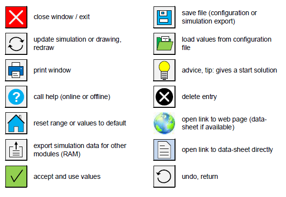
help: This side will appear.

If you have a leased line or a flatrate you should use the auto update. At any program start this update will request automatically. A dialog will opened if a newer version is available. Activate only if you have an always present internet connection!
(default deactivated)

Some firewalls can block the internet  request. Then it is possible after such failed access to try a download of the version file. This file will saved after success in the BassCADe directory and analyze locally.
Try it, if you have problems with updating over existing internet connection. (default deactivated)
Since version 3.2.6 the version info was the last (by Windows saved) value. Versions later than 3.2.7 clear this cache entry before request. Maybe at problem it needs some seconds until timeout.
After the software update check the program compares the number of saved bcd files in sub folder TSP and the numbers on the internet page. If you have less on your harddisk BassCADe asks to go to the web site and download the file.
There you can download the TSP.ZIP and unpack these folders with files into the TSP folder.

Remark:
No data will sent from PC to server. Only a read access (3 files) on the server are necessary for this function.

file export
Additional to the saving of simulation files it is possible to export the results in a CSV file. CSV = Comma Separated Values Here you can modify the format of the ANSI/ASCII file. Excel can open CSV files directly and wants (as the name says) comma separated data fields. Space or semi colon characters are possible in some programs. You can enter each displayable ANSI character. If you want not displayable control characters for data separation you can define the wished
ASCII code (0...255). (default is comma = ASCII code number 44)
Typically these exported files (not the saved one) cannot be read by BassCADe. All numbers are separated by a dot (1.5) as usual in english area. To mark text ranges (begin and end) you can define text identification characters. So a spreadsheet program will assign the complete row to one cell.

Design
Here you can hide some unused buttons or the labels in the main window.

Colors
Here you can choose the colors for the module simulation results comparision. You could select for each of these 6 curves the color with RGB values and select if you want to use a bold line. A black and white background is possible too.
The Grid could have each grey value. With a clock on standard a white background and the colors from formver releases are used. If you select a black background with "RGB default" a usefull possibility is set.


BassCADe configuration files

Since version 3.3.4 you can save the values and setups from many moduls into a file. This file has always the extension bcdcfg. If you do not want to lose data or long search of files you should give your setup a suitable name.

The following modules save additionally all uses TSPs and the simulation results.(maximum one box simulation in a file is possible.)

These both modules save the TSPs of the speaker as well:
If you save data into a existing file all TSPs and the simulation result will overwritten. (Therefore before the question.)
Which data are contained in a BCDCFG file you could see in the module file content file (main menu - help - file content) Here is shown, which modul(s) saved its informations and TSPs and simulation (if existing). All Thiele-Small-Parameters are displayed. Other moduls as e.g. cuboid standing box save only their own data.

It is also possible to open saved BassCADe-Text files (txt, not exported files), to show the saved content of dedicated modles. (also TSPs if available)
If you import the configuration file into a speaker simulation module you can select, if you want to read the TSPs too.

Standing box

In this module you can calculate a classical ashlar box (cuboid) for standing boxes. Additionally the box could have a trapezoid ground for PA speaker.
The inner volume (in liter) is the complete capacity. That means the acoustic volume with additional volume for speaker, crossover, tubes and tunnels. After the selection of width and heigth (in Millimeters) of the box (outer dimensions) the needed
(outer) box depth will calculated The shelf thickness means the thickness (in mm) of the plates (wood etc.)
You can select in which direction you want to calculate. from inner volume, outer volume or all 3 outside dimensions.
Big boxes will get a better stability if you use flat rods (shelves or slats) in each corner. Then you can select this possibility and enter the rod dimensions. The calculation base on that in each corner is one rod.
On the right panel you will get the cutting dimensions of all plates. Depending on configuration of each plate you can choose between six different alternatives. If the opposite plates have the same size only these 6 possibilies are existing.

1) front and back full size, side plates are fit
2) front and back full size, lid and bottom fit
3) lid and bottom full size, side parts fit
4) lid and bottom full size, front and rear part fit
5) side parts have full size, bottom is fit
6) side parts have full size, front is fit

It is useful to plan about 1.0 ... 1.5 mm distance for glue or cut loss. This glue thickness will considered in calculation (0 ... 3 mm, default 1.5 mm).
Depending on selected variant you can see a detailed configuration in a 2D side view (on the right hand) with visible cutting edge. Not visible cut edges are displayed with dashed lines.
Because of the 3 opposite plates three resonant waves will producing The fundamental frequencies will give out.
The flat rods in the corners will not displayed.
With a click on the floppy disk icon you can dave the configuration into a file. You can load a saved configuration (folder icon).

Typical car-subwoofer

Here you can calculate a boy with one slant side for using in luggage trunk of a car. This slant uses the volume behind the back seat.
Further this box has only 2 (not 3) box resonances.
The inner volume (in liter) is the complete capacity. That means the acoustic volume with additional volume for speaker, crossover, tubes and tunnels. After the selection of the above and down depths (in Millimeters) of the box (outer dimensions)
the width will calculated The shelf thickness means the thickness (in mm) of the plates (wood etc.).
You can select in which direction you want to calculate. from inner volume, outer volume or all 3 outside dimensions.
The angle of the slant and its outer height will displayed. For an easier cutting the cut dimensions of all plates will displayed. Here you can choose between 5 different possibilities.

1) front and slant full size, side parts fit (4 miter cuts)
2) front and slant full size, lid and bottom fit (4 miter cuts)
3) lid and bottom full size, side parts fit (2 miter cuts)
4) lid and bottom full size, front fit (4 miter cuts)
5) side plates full size, lid fit (2 miter cuts)

Depending on selected variant you can see a detailed configuration in a 2D side view (on the right hand) with visible cutting edge. Not visible cut edges are displayed with dashed lines.
With the selection of "zoom" you can see detailed the construction of the slant, which is important for the cutting calculation. Before you cut the plates aslope use it straightforward. These cutting dimension will shown dotted in zoomed detailled view.
For instance the version number 1 and 3 are mentioned.
s - slitting width
r - rest


The flat rods in the corners will not displayed.
With a click on the floppy disk icon you can dave the configuration into a file. You can load a saved configuration (folder icon).

Pyramide form box

This box form is rare because it is very extensive. But this pyramide form has a good sound behaviour because construction resonances can hardly occur.
All brinks have to be a miter cut. Dowels and glue gives stability. You can select baseplates with 3 until 16 edges (corners). Upon these edges each side part will positioned. You should not use pyramides with more than six edges.
If you want side parts until below you must extend them. After enterring the inner volume and the inner shelf length the outer shelf length and height (inner and outer dimension) of the pyramide will calculated.
For an easier reproduction the lengths of the isosceles side parts will displayed. Their base side is the outer shelf length. "leg length of triangular shelf" means the both edges which strike in the top.
Because pyramides lose capacity in the top you can calculate a frustum of a pyramide. This (truncated) frustum have the same numbers of edges on the top. For that enter the upper shelf (inner border) length of a side. It must be shorter than the lower shelf length.
So you will get a trapezoid side plate, which one have the lower outer shelf length as basis, 2 legs and the shorter shelf length. The distance between the parallel upper and lower edge will caclulated. (means between basis and top) for an easy line marking line.
To show the assembling in the drawing you can see the side view (one side panel) on the left hand. The top view (cut edges and ground plate) is on the right side.
With a click on the floppy disk icon you can dave the configuration into a file. You can load a saved configuration (folder icon).

Cylinder box

Here you can caclulated bass tubes in cylinder boxes. on the left top you can select the given and calculated dimensions.

t1 is the thickness of the both wooden discs on each end of the tube, t2 is the thickness of the tube around. The min-button sets the minimum diameter of the selected speaker to build it into the disc.

Further data will be calculated.

The drawing shows the view of the circle side on the left and the side of the tube on the right side.

Passive low pass filter

Low pass filters are used to cut off woofers in a crossover. This filter damps higher frequencies stronger than lower frequencies. The order of a filter are defined as degree of the polynomial denominator in the transmission function (frequency response). So a 2nd order low pass filter has a drop of 12dB per octave above the cut frequency.
The wished cut frequency, slope (transconductance) and filter behaviour have to entered, then all needed component values will calculated.
After that with a modification of these values will change the simulation.
The result with other filters you can see in module total X-Over. It is also possible to save or export this result into a text file via the save button.

Behind the filter itself you can simulate a complete crossover part including EQ-parts, attenuator resistors, with measured speaker frequency respnse and impedance response. This is also possible with a simulated SPL response e.g. reflex. For that these values shall be exported into this module before. Only then you can import them here. (Depending on Windows graphics it is needed to click on refresh.)
A click on the picture shows the design of the simulated filter.

advice:
2. order Linkwitz (fc) means the cut-off (limiting) frequency of this filter
2. order Linkwitz is the calculation dep. on the cut frequency of a 2-way crossover.

Passive band pass filter


Band pass filters are used to cut off midrange driver in a crossover.

The order of a filter are defined as degree of the polynomial denominator in the transmission function (frequency response). So a 2nd order low pass filter has a drop of (each) 6 dB per octave above the upper and below the lower cut frequencies. A 4th order band pass has 12 dB on each slope.These filters are expensive and not easily to calculate. Midrage speakers have no linear impedance behavior. So after the calculation and simulation a measurement should be done.
It is not useful to connect successively a low pass and a high pass filter for a 4th order band pass. In the picture is a better combination shown with a absorption circuit (L2-C2) and trap circuit (L1-C1) It has advantages especially in narrow-band filters.
The wished cut frequency, slope (transconductance) and filter behaviour have to entered, then all needed component values will calculated. After that with a modification of these values will change the simulation.
The result with other filters you can see in module total X-Over. It is also possible to save or export this result into a text file via the save button.
Behind the filter itself you can simulate a complete crossover part including EQ-parts, attenuator resistors, with measured speaker frequency respnse and impedance response. This is also possible wit a simulated SPL response e.g. reflex. For that these values shall be exported into this module before. Only then you can importh them here. (Depending on Windows graphics it is needed to click on refresh button.)
A click on the picture shows the design of the simulated filter.

Passive high pass filter

High pass filters are used to cut off tweeter in a crossover. This filter damps lower frequencies stronger than higher frequencies.The order of a filter are defined as degree of the polynomial denominator in the transmission function (frequency response). So a 2nd order high pass filter has a drop of 12dB per octave below the cut frequency.
The wished cut frequency, slope (transconductance) and filter behaviour have entered, then all needed component values will calculated.
After that with a modification of these values will change the simulation.
The result with other filters you can see in module total X-Over. It is also possible to save or export this result into a text file via the save button.
Behind the filter itself you can simulate a complete crossover part including EQ-parts, attenuator resistors, with measured speaker frequency respnse and impedance response. This is also possible wit a simulated SPL response e.g. reflex. For that these values shall be exported into this module before. Only then you can importh them here. (Depending on Windows graphics it is needed to click on refresh button.)
A click on the picture shows the design of the simulated filter.

advice:
2. order Linkwitz (fc) means the cut-off (limiting) frequency of this filter
2. order Linkwitz is the calculation dep. on the cut frequency of a 2-way crossover.

Trimode X-over

Tri mode crossovers are a speacial type for car-hifi areas. On a stereo (2 channels) amplifier is connected with two speaker systems and one subwoofer. This is possible because the 2 power stages are connected in series or a phase is turned at 180 degrees. At a usual home stereo amplifier it does not work. So the subwoofer will controlled only from one channel oder it got the differencial signal, which one contained no bass.
THE CAR-HIFI-AMPLIFIER MUST BE ABLE FOR TRI-MODE!
One sign for that is the bridge function without switch on the same outputs. Depending on the inner circuit is the connection of the subwoofer. Look into the manual an on the amplifier marking! Be careful with the impedance of each system. If the amp is 2 ohms stable, two systems a 4 ohms can be connected on each channel. That means one 4 ohms per channel and one 8 ohms subwoofer in trimode (bridged) together. As in bridge mode the subwoofer impedance will take into both channels. Therefore the woofer impedance have to bisect, if you do not use a passive crossover. A 2-ohms stable amp will work in bridge mode with speaker impedance of at least 4-ohms.

Impedance adjustment

These impedance correction is for linearization of the frequency depending resistance of a speaker. Mainly at subwoofers and woofers strong up- and downturns are possible. First of all it is a rise of the impedance to higher frequencies. The RC element shall work against that. The different resonances occuring with box assembling will compensated with a R-L-C element. It exists one resonance peak in open and contained boxes. For vented constructions one peak will add for each tube.
The values are depending on the resonance frequency and the bigness of this peak. The inductivity (coil) should big as possible, the value depends mainly on electrical quality. Click on the question mark for a useful value.
The inner resistance of the coil is lower than R1 use an external resistor for compensation. The wire thickness should be bigger than 0.5 mm for adequate heating during operation.
The rise of the impedance at higher frequencies are caused of coil inductivity. The compensation with a RC element is important  at passive crossovers connected on tube amplifiers with output transformer.
Housing resonances should be damped with  a suitable construction and wool. The simulation shows the resistance of this circuit. With import of a impedance measurement you can get help for the values. Additionally you can simulate the total resistance of this circuit in parallel with the speaker. It is also possible to simulate only a part of this circuit e.g. only R2 and R3. Suitable values could be calculated by a measured speaker impedance response. Then the corresponding measurement should be imported with "values from impedance meas....". This correction circuit could be simulated with the measured speaker impedance response.

With a click on the floppy disk icon you can save the configuration into a file.
You can also load a saved configuration via the folder icon.


Attenuator (pad)

This part of a passive crossover shall reduce the power of a dynamic tweeter.
bottom:
The real output power of a tweeter (high frequency range of about 2...20 kHz) depends on the input signal and the filter before the speaker. An estimation can made with different spectrums and variable filters. For that the output power (RMS) of an amplifier and the main filter parameter have to entered. So the resulting power in the high frequency range can be calculated.

You can choose from 7 different spektra:
- white noise 20 kHz: each frequency have the same energy
- white noise and harmonic: as above but with some clipping harmonic content with a slope of 12 dB per octave
- music like 20 kHz: untill 1,4 kHz same level, above a slop of 3 dB per octave until 20 kHz
- musik like: as before with additional harmonics over 20 kHz with a slope of 6 dB per octave
- pink noise 20 kHz: range limited pink noise with 3 dB per octave until 20 kHz
- pink noise 100 kHz: range limited pink noise until 100 kHz
- Dance (typical music spectrum)

The last 4 spectrums are user defined and can changed in the options menu.

top:
The tweeter power means the power after the filter. Usually it is in order of magnitude of about 10% of the total output power. (see above) A reducing of the output power on a tweeter after the crossover is only useful with a combination of two resistors. Otherwise the complete crossover has to modified because the one resistor will change the impedance after the filter. So the behaviour of the high pass will changed completely. You can choose resistor values and calculate the new impedance and level correction.

Advice:
At the variant with one resistor will reduce the output power additional cause the increasing total impedance. The calculated value for the power of R3 is based practical on a constant output voltage of the amp. The value in brackets shows the value based on a theoretical constant output power. example: An eight ohms tweeter (after crossover 10 watts) have to attenuate by 6 dB: The calculated pre-resistor R3 must have 8 ohms. The total impedance is now 16 ohms and the output power of
the amplifier is reduced to 5 watts. Therfore the power of R3 is maximum only 2.5 W instead of 5 W.

remark:
This possibility of attenuation will usually not work with a piezoelectric tweeter. In this case a 1st order high pass with high cut frequency (>2 kHz) at an high impedance should used, because these tweeters have a strong capacitive behaviour. So a capacitive resistance must be used. But so other crossover parts are not neccessery. Be careful with inductivities (coils) in a piezoelectric tweeter path. An oscillating circuit could produced.

Equalizer

In this module you can caclulate passive filter corrections. Typical is an attenuation og higher or lower frequencies. An RLC filter circuit can also be calculated. On the left side you can choose a pre-setup with a tip of devices. On the right side you can change these devices and the simulation shows the results. With an imported frequency response it is possible to simulate the impact e.g. to smooth a peak.
With an imported impedance response the simulation results are much better. The checkbox Phase shows the phase frequency response additionally. The both other checkbox show, if the impedance and/or frequency responses are simluated.
Behind the filter itself you can simulate a complete crossover part including attenuator resistors, with measured speaker frequency response and impedance response. This is also possible wit a simulated SPL response e.g. reflex. For that these values shall be exported into this module before. Only then you can importh them here. (Depending on Windows graphics it is needed to click on box "Simulation".)
A click on the picture shows the design of the simulated filter.

Simulation of a total crossover

To simulate the summation of all x-over output signals you have to export (to RAM) the result data of each filter module (low pass, high pass and if wished band pass) before.
Are all needed filter results available you can change the polarity of one output. (typical band pass for 3-way, high pass for 2-way crossovers) Further you can damp the filter channels.
The result is am ideal calculated total sum frequency response. The real frequency response will vary from this result:

reasons:

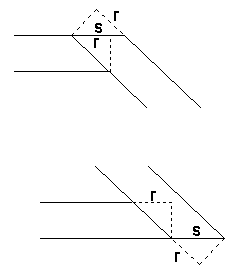
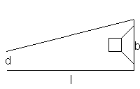
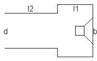
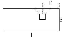
for each filter path you can select:

for the total cross-over simulation:
The home button shows the simulation with default range between 20 Hz untill 20 kHz.

Measurement of TSPs

If you do not have the TS parameters of a speaker you can measure them. The best way to mount the speaker is a small baffle. To get all parameters you have 2 possibilites: 1st mass methode and 2nd volume methode.
for 1st method: after the measurement with a known mass on the membrane you measure the new resonancy frequency. For the 2nd method the speaker will build in a known, contained volume an with a further measurement of frequency an quality you got it.

These steps are neccessery:

1st
At first you have to soften your loudspeaker bead. Use a 15 Hz sinus tone for about 15 hours. The resonance frequency is decreasing. Then let cool down the speaker coil for about 3 hours. So the TS-Parameters can stabilized. After that you can measure the impedance graph.

2nd
Measure with a voltage multimeter the ohmic resistance of the coil. It is a little bit lower than the given impedance Z. (e.g. 3.1 ohms) Enter this value. Measure the diameter of the membrane (pure membrane and the half of the seam. (bead) (e.g. 25.3 cm)

3rd
Replace the speaker with a resistor of 10 ohms and 5 watts. (should be higher than Z) The series resistor should be very higher e.g. 100 ohms. Use an amplifier and a tone generator. So you can arrange the percentage of voltage to impedance and to read the speaker impedance directly.

4th
Then you can adjust the volume level of the amp so you got 100 millivolts at 10 ohms. One useful frequency for this calibration is 50 or 60 Hz. This voltage can be measured exactly by an AC digital multimeter. If possible use and true RMS meter. For all measures use a sine tone.

5th
Connect the speaker with the amp (without 10 ohms resistor). The distances to walls etc. should be high. Then measure the "voltage" depending on the frequency and adjust the generator frequency to get all values. The first value is the resonance frequency the first maximum of impedance. You can draw the measured values in a logarithmic diagram.

6th
The specific measurements you should make exactly and enter these single values in the window. Depending on the sizee of the speaker begin at 15...40 Hz and increase the frequency slowly. You have to look for the first impedance maximum, the hightest voltage... (typical 20...100 Hz) To higher frequencies the impedance will be decreasing... Measure exactly the frequency and the impedance/voltage an enter thes values. (e.g. 30.0 Hz, 260 mV = 26.0 Ohm) This is the free air resonance frequency fs.

Now the software wants to knwo two frequencies f1 and f2  with a special impedance. (e.g. 8.98 Ohm) f1 is the below the free air frequency and f2 is above. Turn down the frequency until the impedance (voltage) reach the given value (89.8 mV for  8,98 Ohms) (e.g. 20.0 Hz) Then look for the upper frequency f2 at 8.98 ohms. (e.g.. 45.1 Hz.) Enter these values. Now the software can calculate the electrical quality Qes, the mech. quality Qms and the important parameter of total quality Qts.

7th
To get the important value of Vas it exists 2 possibilities.
To measure the Vas value, you can use the delta-mass-method, but only with very exact values you got a good result. On the other hand you can use the "volume"-method, but on this way you have got a more complexity measurement. (one second on the other hand a complete impedance graph.)

I prefer the 1st way: Fix an exact mass (e.g. plasticine) at the membrane. The mass itself depends on the membrane mass and should be between 5... 50 gramms. With this additional mass you have to measure the new resonance frequency. It must be lower than the free air measurement before. (in my example a 10 g mass shift the resonance to 28.3 Hz. instead of 30.0 Hz)
Now the software can calculate the Vas (e.g. 124,3 Liter) and some other values.

With the 2nd volume method the speaker is to couple with a known closed volume. Now you have to measure the full impedance curve with new resonance and quality. The new installation resonance frequency and quality are higher than the free air values. Now enter these values and let calculate the parameters.

8th:
The impedance measurement is for coil inductivity Le and you should use a high frequency (typ. 6 ... 15 kHz). Measure the impedance at the given frequency and enter these values. (e.g.. 865 mV = 86.5 Ohm at 10 kHz) Now the inductivity (depending also on Re) will displayed. (e.g. 1376 uH = 1.376 mH)
This parameter is important for crossover calculations, especially impedance correction. Now you can with "use TSPs" accept these values for the simulation modules.

The complete tolerances of all values and results are about 5%, because inexact measurements a temperature rise and imprecise constants e.g. air density and sonic speed. Further series resistance of amp and multimeter have influence of the measurement. If you want the result in imperial units (diameter in inches, Vas in cu. ft, mass, Sd etc.)
you can use the unit-converter
The fastes way to get TSPs is a measurement software as REW. You can import these impedance responses for calculation too.

Import of measurement data


In this module it is possible to import frequency response or impedance curves which were measured and exported with Room EQ Wizard (REW), ARTA or a tool which enerates FRD and ZMA files.

The number of exported values depends on software version and graphic output. For import it doesn't matter the kind of separation type. (comma...)

Now to import click in this module on import and select the specific file (*.txt). You can see the progess during reading and converting. In this window on the right top are additional information, e.g. how many values are read and converted. It shall be more than 900 (min. 96 per octave). Otherwise the curve has too many steps. Better results you will get with more data during export. But you can also select the option "antialiasing", then with interpolation more smoothness will generated. (Therefore select this Checkbox before import.)
BassCADe can only import max. 100000 values. Are more values in the text file you can reduce the number of it with the scrollbar on the left top. Then only each second, third... value will used during reading.
With the checkbox "Phase" you can show the phase response. Especially frequency responses with microphoce could be noisy. Then and averaging of level and phase the results will be better. But less than 1/3 octave is not useful.
Usually the range of 10 Hz...20 kHz will be displayed, The checkbox "full" shows the complete range of 1 Hz...100 kHz.
Now you can select in which measurement slot you will copy the imported curve. Before you should give a good name. You have the possibility for 3 frequency and 3 impedance responses slots. (The phase response will only copied if the phase checkbox is checked and the phase is drawned.) Additional you can copy the frequency response to a box simulation to compare simulation with measurement.
The offset shows the 0-dB line you can adapt before the coping into a slot. The lowest and top frequency could be changed tu cut the frequency range.
The imported measurement (before copy-to-slot) caould be extended. Then the old border value will be used until the new wanted limit.

Maximum Sonic Pressure

Because the human ear works logarithmic, for many people it is hard to imagine what loudness will generated with pairs of speakers. That's the reason, why all calculations were made with the logarithmic "dimension" decibel (dB). For better understanding the new dimension sone (loudness) was introduced. A double sone value means a double loudness.
1 sone = 40 dB, 2 sone = 50 dB, 3 sone = 56 dB, 4 sone = 60 dB.
In the unit calculator you can convert these dimensions.

For a double loudness the level must have factor 10! (+10 dB). That means factor 10 of the output power too! A double sound pressure effects only a gain of 6 dB.

Further you have not the double sound presure, if you use 2 same boxes. The level gain (addition of RMS values) about 3 dB. That means you need 10 loudspeaker boxen with the same loudness for the double loudness!
Only if both speakers (with double membrane surface) give the same signal with same phase and their distance is very shorter against the wave length of the signal you will got a level gain of 6 dB. This works only with parallel connected and closely mounted woofers.
This calculation based on boxes which are separated by open ground, so the RMS values will added. With selecting of "add pressure" it is possible to calculate with +6 dB with double speaker number e.g. in the bass frequency range.
With a double distance to boxes the sound pressure will reduced at 6dB. Only with a line-array only 3 dB with doubeling can be achieved This option you can select with r (r²).
These decibel values define a level which is independent on frequency. However the human ear hears different frequencies with the same level with different loudness. The dimension unit "phon" will correct these influences. It is possible with isophones curves based on the same loudness. The correlation between phon and decibel shows a special diagram (acc. DIN 45630). How to see at 3.5 kHz only 115 dB reach for 130 phon (achiness threshold). In the low bass range (about 30 Hz) you need about 150 dB for that, factor 60 of sound pressure.


(source Fellbaum, Klaus: Elektronische Sprachsignalverarbeitung)

A sound pressure measurement with a real loudness is not so easy. Therfore simply curves (A, B, C, D) will used to prefilter the signal. the unit is then e.g. dB(A).

One advantage of the logarithmic calculation is the large range. And a conversion of a multiplication to an addition.
10dB + 10dB = 20dB means 10x power * 10x power are 100x power

Because of coil heating by powering, the received electrical power is decreasing. So the acoustic power is also smaller than with lower temperatures. You can calculate this effect. For estimating of coil temperatures depending on electrical power
some experienced (boy type) from PA are used.

New (since version 3.4) is the possibility to calculate the needed piston excursion depending on wanted SPL.

On the right hand the frequency-depending absorbtion could be calculated depending on temperature, air moisture and aire pressure the additional freq. dep. absorbtion.
In air the higher frequencies are absorbed with higher intensity than lower frequencies.

Interference

This module shows the SPL in a room as sum of two sound sources.
For that purpose the wished frequency or wave length must be defined. The wave length depends on sonic speed (at same frequency). This speed is depending on air temperature. The sonic pressure level (dB in a distance of 1 meter) an phase shift (typ 0 could be in a range of -180...+180°) e.g. after crossover parts or if a speaker has an inverse polarity (180°).
Right hand of the graphic the distance of both speakers to the beginning of simulation (-20...-100 cm) and the distance to each other (3 ... 450 cm) is defined.
With tlhe scrollbar below you can change the resolution of the calculation of graphic output. At 1 cm resolution more than 230,000 points must be calculated. With lower resolution you can increase the calculation speed.
On the right hand a graphic shows with a (selectable in the middle) color system the SPL in a 480 x 480 cm room (without walls). An identical color means a similar pressure (2 dB resolution).A cursor on the graphic shows further information to this position. This are the position (X width, Y depth), the distance to the left and right speaker, the relative SPL (acc. to the loudest of both speakers) and the absolute SPL in dB. With a click in this area both distances are taken for the single calculation. Then on this position the entire listenable frequency response will be shown (if checkbox selected).

With a click on the floppy disk icon you can save the configuration into a file.
You can also load a saved configuration via the folder icon.

Volume correction

One part of ths calculation was in former versions in modul tube calculation.
For the calculation of the needed inner volume of the box the following volumes will be considered:
- acoustic volume (directly from the speaker simulation)
- "win" of volume because of damping material (insulation)
- displacement volumen from the speaker itself
- additional volumes for internal boards or crossover parts
- additional volume(s) because of reflex tubes or tunnels

This modul can called directly in the box simulation moduls (contained, reflex, sealed band-pass, vented band-pass). Then all data will be transferred into this module. Now just modify the thicknesses of wall, tunnels or tubes.

The position of the tube or tunnel has an influence on the volume. Here you can select of 8 different variants to calculate the needed internal box volume. The new really needed inner volume is shown, you can directly transfer is the wished housing module.

Advanced tube calculation

This tool can called by the main window or from a vented module. (one click on tube diameter)

upper left: minimum tube diameter
After entering of the needed values an advice will displayed with the dimension of the inner tube diameter. Depending on the membrane surface, Xmax and the tuning frequency the recommendable inner diameter will calculated.

upper right: tube length transformation
The tube length of a vented system is dependent on mounting. Do you want another positioning with mounting you can correct the length.

In this software (as in other programs too) the tube length is normed. So the tube is flush with the outer plane and extend free into the inner volume. (see image upper diagram)
The tube can shortened if it flush on both ends. This length can be used for pure box plane cuts without tube too. (image: middle)
To allow very long tubes the tube can protrude of the box. But so it must additionally extend. (image: below)
This transformation is important for big tube diameters, otherwise the tuning frequency are not correct. right below Tube to tunnel calculation (and reverse) Do you want to use a tunnel instead of a tube, you can let calculate the dimensions.


below: tube length recalculation
Are the diameter and the length of a tube given from the manufacturer, it is possible to calculate the tube length with a different diameter. For a bigger tube diameter a longer tube is needed. But this ratio is not linear.
You can select between the linear way and the complete way with air-column correction. Linear means length depending on cross-section of tube. But resonating air outside the tube changes the tuning frequency, so the tube can be shortened in real...

Depending on the installation of the tube the k-factor changes, which defines the shortening depending on the diameter. Typically it is 0.732 for a standard tube (upper figure), which is also used in all simulations.
But the k-factor could be dep. on tube design and installation in a range between 0.45 and 2.23. Second image k=0.85; Third image k= 0.614

Top in the middle: Tube to tunnel calculation (and reverse)
Do you want to use a tunnel instead of a tube, you can let calculate the dimensions.
Attention: A change of the amount of tubes/tunnels will change the tuning setup even if the total cross-section is the same!

right below:
To suppress a standing wave inside the housing, an integrated Helmholz-Absorber could be used. A hole in a partition panel has the same effect as a reflex tube, but it works against the resonance.
With a definition of inner interspace (wavelength and so direct the disturbing frequency), the partial volume the dimensions of the hole are calculated.

Determine the loss factor Ql

It is useful to check the tightness of a reflex box construction. So you can get an estimation of the differences between construction and simulation. The estimated Ql value e.g. 10 can measured now.

1st Enter the Thiele-Small-Parameters (Qts, Qms, Qes, fs)
2nd Measurement of the frequency at the lower impedance maximum fl and entering
3rd Measurement of the frequency at the upper impedance minimum fm and entering
4th Measure the resistance at impedance minimum Rm and enter
5th. Measure the frequency at the upper impedance maximum fh and enter
6th. Seal the reflex tube (close to be airtight)
7th Measure the resonance frequency of the one impedance maximum of this closed system and enter

All values will be calculated now. The quotient of fb/fm is needed to estimate of the deviation. It should be about 1. The tolerance will displayed in per cent. All values smaller than 5 percent are very good.

Displacement

The displacement ist the volume of the speaker which one get lost the acoustical behaviour. To calculate the displacement volume of a speaker you have to enter typical dimensions. After input of all dimensions the displacement will displayed. With a click on the "accept" button this value will used for the currently defined loudspeaker.
In this picture the blue part shows the cut through the front panel. All values d1...d5 are diameters (in millimeters). The length s, the width and thickness are bridges (webs) of steal plate or aluminium cast. These webs hold the chassis and connect the magnet with the front.
This volume depends on the assembling of the speaker. The usual front assembling means the screwing of the speaker on the outside of the front panel.
The displacement will increasing if the speaker are screwed behind the front panel. So you can see the cut of the panel. This mounting is needed for some speaker types. Select the mounting type with the check box for correct calculation.
Additionally it is possible to use the show-car-woofer-variant with basked outside. Her you will get a negative volume because of the won capacity between membrane and box housing.

How to connect many loudspeakers

If you want to connect many boxes or speakers together on one amplifier output you have different possibilities, The classical in-series circuit and the parallel connection. With more than 3 speakers you get further options.
Do you connect to many speakers parallel the total impecance will decrease. So the amplifier cannot control this load. Sometimes a damage of the power stage is possible. Do you connect to many speaker in series (sequential) the total impedance will increasing. So the output power of the amplifier could be too little. The system is not loud enough.
Is the number of speakers 4, 9 or 16 it exists options having the same total as the single impedance. In this module all variants will calculated at each speaker get the same power.
The picture shows a variant with 6 speakers. Here 2 speakers are connected in series. These 3 groups are connected parallelly. With a speaker impedance of 6...8 Ohms the total impedance will be higher than 4 Ohms.
Use only absolutly same speakers for these connections!
The simple parallel connecting of more-way speaker boxes will work. Look after the total impedance of speaker and amplifier! You shold not connect different more-way speaker boxes because the impedance will changing over the frequency.

Winding of air coils

Air coils can be made easily by winding. Maybe if you could not buy a special inductivity. With targets of inductivity and serial resistance this software calculates a typical core diameter, the coil height, the number of turns and the wire diameter.
In a range of 100 uH until 1 mH this standard calculation should work. The DC resistance can be estimated depending on the (woofer) loudspeaker. So a maximum installation quality will be allowed.
standard core:
The core diamter is the double height.
small core:
Better use this type only for kHz range. The core diameter is 4 times bigger than the height.

This results are only guiding values (targets)! After the winding the inductivity must measured and where necessary change the numbers of turns.

For confirmation of right inductivity you should measure this value. Here you can enter the measurement values to get the calculated inductivity. The best method is as serial resonance.

Unit converter

This module converts for instance metric (SI) to anglo dimension units and back. So parameters of US manufactors can be converted and entered in the TSP input window.
Select the given unit and enter the value, then the software caclulates this value from this dimension to all other units.

length...volume
You can enter the length in foot and inches (german: Zoll). (12 in = 1 ft.) If you enter a bigger length than 1 ft.then a mathematical and the ft/in will be shown. You can select the inch in fraction type. Then you can enter a "3" in the first cell and  "3/4" in the second one instead of 3.75. This length converter tries to calculate a value into fraction type. Maximum divider is 12. If you reach the exact fraction value or only an estimation is shown with the ca. value (round).

A conversion of a cubic dimension is possible into dry measure and liquid measure.

There are differences between english/british (imperial) and american measures. All dimensions in this converter tool are US units!
1 US gallon = 3,79 liters
(1 imp. gallon = 4,55 liters)

Level:
Here is the conversion of decibel sound pressure level to sone and the absolute pressure in Pascal possible. The ratio (amplify or damping) of voltages (or related field variable) and power (or other energy dimensions) will calculated. Be careful: The user have to know what kind of conversion shall calculated! Do not mix absolute and relative level specifications!
With pressure in Pa and with ratios of voltage and power the metric prefixes will used:
factors:

f (femto) 10 to the power of -15 (quadrillionth)
p (pico) 10 to the power of -12 (trillionth)
n (nano) 10 to the power of -9 (billionth)
u (mikro) 10 to the power of -6 (millionth)
m (milli) 10 to the power -3 (thousendth)
k (kilo) 10 to the power of 3 (thousends)
M (mega) 10 to the power of 6 (millions)
G (giga) 10 to the power of 9 (billions)
T (tera) 10 to the power of 12 (trillions)
P (peta)  10 to the power of 15 (quadrillion)

On the right hand dBu, dBm (=dBmW) could be calculated into voltages and back. Both Ohm values relates to the dBm values left and right. 1 dBu = 1 dBm @ 600 Ohm.
On the bottom side AC voltage values (Urms, Up, Upp) could be calculated to the crest factor.

frequency, time:
On the right side you can calculate periode times and frequencies to wave lengths. The time of sonic into distances can be calculated too.
Down below a calculation is possible in which distance a cylinder wave (e.g. from a line-array) has a transient to a point source (spherical  wave).

Frequency, Q::
Here the center frequency, the quality Q, bandwidth and lower and upper cut frequency of an oscillating system can be calulated to each other.

Mass, temperature:
On the left different mass units (weights) could be calculated to each other. On the rigth a conversion of different temperature scale values is possible.

Interpolation:
To determine points on a characteristic curve (e.g. table values) this can be done by interpolation. Lineary and logarithmic interpolation need 2 nodes (x1, y1, x2, y2) and an xi preset value to calculate the target value yi. For logarithmic interpolationd only positive values (>0) are possible.
For square interpolation (polynominal 2nd order) needs 3 and cubic interpolation (polynomial 3rd order) 4 nodes. These preset values x1..x4 must be in increasing order.
Average values of X1 and X2 are calculate below.

Music:
On the left the beat (measure) is converted to time intervals. BPM=beats per minute, BPS=beats per second.
With a click on the tap button you can count the time and cklicks to calculate the BPM. Recommended is a number of at least 20 clicks.
hint: the measurement is performed in a 100ms timer. Windows iss no real-time operating system (RTOS), so the result can dither.

On the right hand you can calculate the frequency of all notes depending on A (usually 440 Hz)
The german and english notation is shown.

File size:
The calculation of the size of an audio file depending on run-time and data rate is possible on the top. The data-rate can be defined directly (e.g. 320 kbps=kilobit per second) or taken from LPCM signals (uncompressed) dep. on channels, sampling-rate and resolution. Some presets (e.g. CD, DAT) are available for that.
Below the uncompressed image file size and (height-width) image-ratio could be calculated. For that horizontal and vertical resolution in pixels and the PAR pixel-aspect-ratio (ratio width to heigth of a pixel) values are needed. The DIV value shows the maximum divider based on 2 (up to 256) of each pixel numberwill also given. The most video compressors requires at least 2 (even number), but they work better with values of 8 or 16. The color depth is typical 24 bit (3x8 bit RGB true color), but also 16 bit (e.g. YV16) or higher values (32...48 bit) for HDR pictures are used.
Addionally you can "calculate" a random number in the defned number range.
The limit is a decimal number with 17 digits, this is a 55 bit number.

ADC:
To calculate voltage values of ADCs (Analog Digital Converter) e.g. in micro-controllers, here the maximum value and the resolution is given. MC internal ADCs have often only 8, 10, or 12 bit, better measurement systems 14 or 16 bit. Audio system do a sampling with 16, 20 or 24 bits. Maximum 32 bits are possible.
Is a voltage divider in front of the ADC input (e.g. 32.768 are decreased to 5 V) this wanted or real maximum value can be selected to calculate a 12 V input voltage.


RMS:
In the "RMS" section it is possible to calculate RMS (rroot mean square) or average values for definable, periodic signals.
To understand the results I used the following equations for the calculation.
(A description you can find in wikipedia.)

RMS formulas

On the right side you can select some default signals. It is also possible to define a signal by yourself. The maximum peak voltage value and the signal curve in % of time of a periode and in % of max. peak voltage are defined.
The first value must be always 0% the final one at 100%. Here only integer values are allowed in decreasing order. The voltage values must be in a range of -100 ... +100%. So up to 101 rows (each 1%-steps) are possible.
Does the signal contain non-linear fnctions eg. a sine, then the results will only leads to an approximation.
On the right hand you can select from different presettings. The saving and loading of the signal definition (table values) could be done into a BassCADe configuration file.

DMX:
In Tab "DMX" on the left side an assigning of a DMX-address to a dedicated channel of a bank could be done. On the right side a calculation of DMX-address into DIP-switch positions can be performed or vice versa.
DMX supports from the first up to channel 512. To adress single-channel devices to this final channel with only 9 DIP-switches, it is possible to use adress 0 or the entire range is shiftedby 1. This means DIP=0 represents channel (adress) 1 and DIP=111111111 = 512th channel. This shift can be selected by the checkbox "Addr.=DIP+1" on the right.
Right below you can calculate a color definition for a LED spot (RGB, RGBW or a different light effect device). The definition for (R,G,B (W) is usually represented by different DMX channels, each of them has a range of 0 ... 255.
You can choose to mix a white channel additionally.

Car-HiFi power wiring

In this module the neccessery cross-sections of power cable are calculated. These cables are for Car-HiFi amplifiers (power stages).
You can select up to 4 different amplifiers. Each amp could have up to 6 identical channels.
1st step define each amplifier:
Here you can enter the maximum supply current or the total nominal power or the RMS output power per channel (RMS) with an estimated degree of efficiency.So the max current to each amp is known. With a double click you can enter a name to each amp.

2nd step enter wire lengths:
Do you want to use more than one amplifier a power splitter have to use. Please enter the length for each cable. Any amplifier with its values can be saved to files. The saving of the complete configuration is possible. Then voltage drops will calculated. These drops are depending on ground cabling too.
With these total currents each minimum cross-section will defined. (with Tip or Auto-Tip) The calculation base is a DIN norm: group 2 with more parallel installed cable in one conduit.)
With "upper limit layout" all cables and fuses will use up their maximum. The best way is a spare (reserve). So fuses will not disconnect too fast.
You can modify each cross-section, the numbers of wires and the fuse value. Each cable must have a fuse for its own. Will determined a departure from the norm (maybe too high current for cable) a red note of exclamation will appear. In the below status bar the reason will displayed.

Electronics modules

Since version 3.4.4 diffferent electronics modules exist. These ones can be opened only via menu not with a button.

1. RC-Filter

In this module different simple, passive RC-filters (lowpass, bandpass, highpass, RIAA-filter) could be calculated and simulated.

At first on the right hand the type of filter shall be selected. Then the matching schematics is shown.
possible are:
-RC-lowpass: RC standard filter
-RC-highpass: RC standard filter
-RCR-lowpass: standard filter incl. voltage divider (e.g. for ADC's)
-RCR-highpass: standard filter with subsequent voltage divider
-RC-RC-lowpass: Two direct subsequent RL low pass filters
-CR-CR-highpass: Two direct subsequent RL high pass filters
-CRRC-bandpass: highpass with subsequent lowpass
-RCCR-bandpass: lowpass with subsequent highpass
-RIAA standard: ideal resistance network for phono de-emphasis
-RIAA real: resistance network for phono de-emphasis with components of neighbor stages

On the right side below you can select the type of simulation:
-G(f) is the frequency response (Bode diagram) optional (°-checkbox) with phase response *
-rising edge (step response) with constant (0 ... 10) Tau (Tau is the time constant which equals R*C at standard filters)
-rising edge (step response) with selectable time range (10 us ... 10 s)
-falling edge (step response) with constant (0 ... 10) Tau (Tau is the time constant which equals R*C at standard filters)
-falling edge (step response) with selectable time range (10 us ... 10 s)
-sine curve with selectable frequency as input signal (based on one periode)
-sine curve with selectable frequency as input signal with selectable time range (10 us ... 10 s)
There are not all simulations implemented for all filter types.
The cursor shows in window title the corresponding coordinates in X- and Y-direction.
If the left mouse button pressed the curve value (voltage, level) iself is shown on selected X-position.

* With this simulation is is possible to simulate decoupled sequentially filters.
The button on the right is for export, use it. With "used saved response as input" this saved curve can be used together with ther current filter.
Up to 12 of these steps are possible. Each one will shown in the main window.
The saved export can be shown additionally by selecting of the checkbox "Filterexport".

Via scrollbar you can choose which frequency or component values shall be defined or calculated.
The input voltage Uinp is the peak value. "U RMS" is the AC value. Via this checkbox you can select which one you want to enter.
On the left all needed component values are shown. You can modify these ones directly or indirectly. The simulation below will be adapted.
With a double-click on one of the underlined units you can change it. (u means mikro)

RIAA:
This RIAA filter is a passive RIAA-network.
It is needed to de-emphase the analog signals of a record player.
Base is the reference plot of the RIAA with the three time-constants 3180 us, 318 us and 75 us.
Due to influence between them here new ones are used for this circuit: 750 us, 318 us and 109 us.
You can show this reference plot for comparison with the checkbox "show RIAA reference response".
RIAA-Standard is the pure RC-network, RIAA-real contains selectable the output decouple capacitor C0 of the previous stage and the input resistance R3 of thenect stage.
These ones affect the behavior esp. in the lower frequency range.
With pressed mouse button additionally to the voltage and dB the difference to the reference will be shown.

With the advice-button (lamp) you can try to find better result with both RIAA-filters and two subsequent RC filters based on the cut frequency.

With a click on the floppy disk icon you can save the configuration into a file.
You can also load a saved configuration via the folder icon.

The shown simulation (time or frequency) could also be exported (floppy icon) to a text file.

2. Vacuum tube amplifier

Here an pre-amplification stage could be calculated. On the top right hand the main characteristics like gain, transconductance, serial resistance could be calculated. The wanted value should be selected. Depending on supply voltage on the anode the surrounding resistors all outcoming values
will be calculated.

3. OP amp

In this module an OP amp stage could be calculated At first it should be selected if an inverted or non-inverted circuit shall be used. After that the user selects which 3 of the 5 parameters are given. (8 variants) Input voltage U1, output voltage U2, resistor R1, resistor R2 and gain are possible. (calculated values are grey) Each voltage can be entered or calculated in mV or Volt. Resistor values are possible in Ohm or kOhm, gain as factor or as decibel value. To change that a double-click on the unit will change it.

To estimate the maximum gain depending on the upper cut frequency the right block below can be used. You select if you want to calculate the gain or the upper frequency. These values depends on the bandwidth and the open loop gain of the OP amp itself. For some often used types are values given.

4. Standard applications (Electronics)


4.1. Series resistors for LEDs

At first the wanted value should be selected, usually it is the resistor. Then the LED type should be picked to define forward-voltage and LED current. (Of course the current if its value should not be calculated.)
Depending on power supply voltage U, the number of LEDs in series (see fig. 2) and the load current the resistor will be calculated. With the button "max?" tha maximum number of possible LEDs will be used. This depends on supply voltage and forward voltage.
Additionally the power dissipation of resistor and LED will be calculated.

4.2. Transformer power supply

On the top the maximum achievable DC voltage could be calculated from the AC voltage. The standard is the bridge rectifier with 4 diodes. Optional for low loads a simple half-wave rectifier is possible.
In the bottom part the voltage drop is calculated depending on the capacity and load. The following 3 different load types are considered.
 resistive load (voltage decreases via exp function)
 constant current (linear drop)
 constant power (e.g. DC-DC-converter) with quadratic fall

The voltage will be simulated over time for a half period. (for the half-way rectifier a full periode)

4.3. Adjustable voltage regulator

Here the classic voltage stabilisation with an regulator from the LM317 series can be calculated. The wanted value (usually R2) should be selected at first. After that all other values are entered. The ratio of both resistors defines the output voltage.
A double-click on the underlined ratio will open the module, which calculates different resistor values depending on this ratio.
R1 should be around 200 Ohms, but must be less than 1 kOhm. The resistor R2 can be entered in Ohm or in Kiloohm. To change the unit you need to double-click on the unit.
With both scroll-bars of reference voltage and ADJ leakage current you can simulate the tolerances.
The variante for negative voltage LM337 could be calculated in the same way, only the circuit is a litle bit different.
The main LM317 calculation will also work for similar regulators e.g. LM117, LM217,  LM1084-ADJ, LM1085-ADJ, LM1086-ADJ, LM-1117-ADJ, LP3965
The main LM337 calculation will also work for similar regulators e.g. LM137, LT137A, LT337A

4.4. Oscillator circuits

The generate a simple clock in a range of some Hertz up to many Kilohertz, here are some possibilities with flip-flop / multivibrator circuits. Be careful with the high tolerances which occure usually with these circuits.

4.5 Zener Diode (ZD)

To limit a voltage a Zener diode can be used. The input voltage is higher and the zener voltage is the output voltage. The needed voltage drop will be created by the resistor R1. Its value depends on the minimum and maximum load current. Often problems because of too high power dissipation in R1 and ZD occur.
You can define the minimum and maximum load case, either as resistor load or constant current. With a click on button "R1" an estimation for the value of R1 will be done. This resistor limits the load current. The load current is too high if the output voltage is less than the zener voltage.

4.6 Real power supply

To consider the internal resistance of a voltage supply or to calculate the output voltage at different loads you can use this tab. Via scrollbar it is possible to select which values shall be defined and which one are calculated.
U0 is the open-circuit voltage (max. voltage without load). Isc is the short-circuit current, the (theoretical) maximum possible current with a zero output voltage. Ri is the internal resistance of this power supply.
UL1 is a arbitrary voltage at a load resistance RL1 with a load current IL1. UL2 is a (from UL1) different voltage under load of resistance RL2 and current IL2.
With a double-click on underlined units each voltage can be switched between V and mV, each current between A and mA and each resistance between mOhm, Ohm and kOhm.

5. Resistors

In this module you can do the following:
  4.1. translate SMD marking codes to real values
  4.2. transfer color marking codes to value and tolerance
  4.3. calculate the resistance of parallel and serial circuits of up to 3 resistors
  4.4. caclualte voltage, current, resistor and power according to Ohm's Law
  4.5. Ratio of 2 resistors: Search for matching resistor pairs depending on a given ratio or from a voltage divider


5.1.
Excluding the value 0, different combinations of 2 or 4 characters could be entered to translate them into the value e.g. 102, 1001, 01B (each means 1 kOhm)

5.2.
On Thru-Hole resistors are color rings or marks. The reading is from left to the right side. To recognize the left side all rings are mor on the left as on the right hand or the last ring has a larger distance to the former one.
At first the number rings must be selected (3...6) with the up-down lever. After each color is chosen the resistor value with its tolerance will be shown.

5.3. Series, parallel circuit
At first you should select if you want to use 2 or 3 resistors and a series or parallel circuit. Now you can choose you want to calculate the total or a part resistor. With a double-click on the unit you can switch between Ohm and kOhm.
Hint: to get more digits after the dot add more digits on the input values, e.g. "10.00" instead of "10".

5.4.
Here 2 values (voltage, current, resistance, power) could be calculated into the other both ones acc Ohm's Law. For that change the scrollbar the wanted values. (grey)
With a double-click you could change each underlined unit.

5.5.
Here you can calculate resistor pairs depending on a given ratio.
The first possibility is from a voltage divider. To achieve the wanted output voltage from the input the voltage ratio (default 25.5 V -> 5.0 V, -> 5.1) and the resistor ratio (->5.1) will be calculated. With the given decade range of resistor R1 matching R2 resistors will be searched.
It can be selected if E24 or E96 row (or both) shall be considered. In the table below all resistor values in the decade are shown with matching R2. (sorted acc. R1 value or ratio tolerance)
Also shown in the table is the sum R1+R2 and the max. power dissipation of one resistor.

The second possibility is to define a resistor ratio as fraction e.g. 9/4 (=2.25). A calculation of power disspiation is not possible in that case.

The third variant is a directly given ratio with a voltage.
The 1/x button will set the ratio to its reciprocal value. (e.g. at 9/4=2.25 -> 4/9=0.444)


6. NTC's

In this module thermistors / NTCs (Negative Temperature Coefficient resistors) can be calculated.
The calculation is based on the Beta- (gradient) and R0-value (resistance at 25°C). On the left hand you can calculate resistance to temperatures or voltage and vice versa. The voltage based on a resistor divider, so also the calculation of ADCs values on a micro-controller input is  possible. The result is shown as graphic curve, selectable is a lineary or logarithmic Y axis. This diagram helps to select a suitable resistor for the NTC.
Hint; A high power consumption of the NTC itself will lead to an additional temperature rise and deviations on temperature measurement.
In tha table on the left you can see the calculated values in steps of one degree. (NTC resistance, output voltage and ADC value) The lower temperature (-60°C ... 0°C) can be selected with the left and the upper temperature (80°C ... 200°C) with the right slider.
For the ADC you can chose 8 ..20 Bit resolution, typical are 8, 10 or 12 Bit inside micro-controllers.
The data inside the table can be exported as text file via the save button. It is also possible to save all data into a bcdcfg-file.

7. Capacitors

7.1. here you can calculate the total capacitance of capacitors in-series or parallel circuit
7.2. marking of capacitors
7.3. replacement values
7.4. calculation of reactance and inductance of coils and capacitors

7.1. Series-, parallel circuit
At first you should select if you want to calculate 2 or 3 capacitors and if you have a parallel or in series circuit. Then you select if you want to calculate the total or a partial capacitance.With a double-click on the underlined unit you can switch between pF, nF and uF.(micro-Farad)

7.2. marking of capacitors
Here you select the type of capacitor and the printed code. Then the capacitance and if possible voltage and tolerance will be shown.

7.3. replacement values
In the center part it is possible to calculate alternatives for a target capacitance. For that purpose additionally to the nearest standard value some combinations of standard capacitors connected  in parallel or in series, which are close to target value. With a double-click on the underlined unit you can switch between pF, nF and uF.(µF or micro-Farad)
The number of decades represents the ammount of combinations. The default value 2 decades means one decade (e.g. 1.2 nF ... 10 nF) also the next decade (120 pF ... 1 nF for parallel connection) will be calculated to find more combinations..

7.4. Impedance, reactance, inductance
Here you can calculate the complex impedance of capacitors in combination with coils and resistors. You can select beweeen a parallel and a series oscillator circuit. The calculation could be made with an internal resistance Ri of the coil L. The impedance could also be calculated with L=0 and Ri=0.
With a double-click on the underlined units you can switch between differen ones.
The button "Res" could be used to calculate the resonance frequency if L and C are greater than 0. In this case the complex part of the impedance is zero.
Both parts (Re, Im) and the absolute value (abs IZI) of this complex impedance Z, the phase angle phi and the power factor cos(phi) will also be shown.
If you want to calculate without the coil you can use the "X"-buttons to set the resistor or inductance values to values without influence.

8. PCB (printed cicuit board)

This module was taken from my old PCBtherm software and integrated into BassCADe.
In the upper left part you can calculate the width of a PCB track depending on current and heating. The model of the industial standard IPC-2221A is used for that.
It covers the following ranges:
At first you select which value you want to calculate. (usually the width) Now you enter the maximum ambient temperature and the allowed temperature increase. This maximum PCB temperatur shall not exceed the tg-10K (glass transition temperature). The copper thickness (usually 35 or 70um) and the current determine now the minimum width. The length of the track is only relevant for the voltage drop. This one will also shown with resistance and power dissipation. Copper thickness, temperature difference, track cross-section and current density will also shown in US units.

Additionally to this IPC standard for permanent currents an energy related calculation could be made. For that the energy (power and time) will be considered which ones will heat the existing copper mass.

In the part below you can calculate the needed number of vias depending on dimensions and current. Here you select what shall be calculated too. (usually the number or the drill diameter)

In the right hand the minumum distance between 2 tracks for insulation depending on the voltage.

9. Cooling of devices and heatsink

In this module you can evaluate the temperature of electronic components due to their power disspiation. On the left hand it is possible for SMD (Surface Mount Device).
Usually the maximum ambient temperature is defined. Only the thermal resistors Rthja (junction to ambiant) and Rthjc (junction to case) have an influence on the temperature difference depending on its power dissipation. Often you select if you want to calculate the maximum power dissipation inside the component or the arising die temperature. Different housings have specific Rthja values, which are mentioned in the data-sheet of the device.
If you do not want to calculate Rthja you can choose a dedicated package on the top ("SMD package") Depending on the allowed temperature increase you will get the power dissipation value or vice versa. The temperature gradient inside the package based on the Rjc (junction to case) will also be calculated, because high values will lead to a reduced life-time.

On the right hand the temperature caclulation will be made for standard thru-hole devices (THD). It is possible with and without an additional heatsink. For standard devices without a cooling area also the Rthja value will be used if "use heat-sink" is disabled.
The temperature difference between silicon (die) and ambient will be determined of the thermal resistance Rthja2  (junction to ambiant) and the power dissipation inside the component.

With additional cooling ("use heat sink" is enabled) the different thermal resistors must be entered. If you do not want to calculate Rthja2 you can choose a standard THD packages on the top ("THD package")
 Rtjc2: is the thermal resistance from junction (die) to case surface. This value is inside the data-sheet.
 It is also possible to calculate the maximum needed value depending on all other values.
 Rtch: It is the thermal resistance from case to heatsink between the component and the cooling part.
 Heat-transfer-paste or insulation washer will influence this value.
 Rthha (heatsink to ambient) is the thermal resistance of the heatsink itself. A larger heatsink has smaller values.

10. Cables and wires

In the part on the bottom you can convert the American Wire Gauge (AWG) system to the linear metric system in cross-section (mm²) and diameters and vice versa.
A summarize of more wires is possible: 3 wires AWG 12 are which one wire diameter?
You can enter the dimension of big wires in AWG as "3/0" and "000".

On the left the given values of one wire and unit should be entered, the scrollbar is for the number of parallel used wires. Then all other units will be calculated for one and for all wires.
On the right hand you can also select a unit or the numbers of new wire types. ("number" is enabled") e.g. 1 wire with 1.5 sqmm will lead to 5 wires with 0.35 sqmm (calculated 4.3).
This part was in former versions (until 3.4.3) in the unit-calculator module.


Top 1st silde: speaker line loss
This part was in former versions (3.3 until 3.4.3) in the module "speaker interconnection". You can calculate the loss of power depending on speaker cable length and diameter.
Depending on calculated current the minimum needed cable cross-section and the loss in decibel will be shown. This minimum cross-section shall not fall below this limit, otherwise the cable will be overloaded.

With this serial resistance the contained quality Qtc will increased and will lead to a changed bass characteristics of the speaker.
The voltage drop over the cable due to current is higher with lower speaker impedance. Of course the loss will be higher with a longer and weaker (thinner) cable.


Top 2nd slide: loss of wires

Such calculation of cable loss can be done in general for all types of wires and cables. Depending on the material (usually copper, but also aluminium etc.) with its conductance, the cross-section and the length the resulting resistance will be calculated.
The checkbox "x2" should be used for a twin-wire cable with go- and return line. This means one cable with e.g. 10 m length with resulting 20 m total length.
With a double-click on the underlined unit you can switch between ohm and milliohm and between meters and millimeters.
On the right hand the voltage drop and power loss will be calculated depening on this resistance, supply voltage and a current due to a resistive load


Top 3rd slide: cable capacitance
For AF and RF cables the cable capacitance has a big influence on the upper cut frequency. The maximum achievable frequency which can be transmitted will be lower with a higher specific capacitance, a longer cable and a higher series resistance of the transmitter.
The wire inductance and resistance will be ignored here. You can choose between 3 different types of cable: a simple coax (e.g. cinch-cable), a twin wire without shield (e.g. speaker cable) and a balanced shielded cable like PA or studio microphone cable.
With a longer cable (e.g. 35 m) it is not possibe to use a mikrophone with high impedance (e.g. 5 kiloohms) because the frequency response will be restricted in the speech range. The reachable upper cut frequency must be obviously higher than 20 kHz.
At this cut frequency you have a high phase shift which could lead for instance to problems with large rooms and many microphones on a stage.
After you have selected the value you want to calculate you have to enter the other ones e.g. the specific capacitance values and the length of the cable to get this cut frequency.

wire thickness:
Here you can convert the American Wire Gauge (AWG) system to the linear metric system in cross-section (mm²) and diameters. A summarize of more wires is possible: 3 wires AWG 12 are which one wire diameter? You can enter the dimension of big wires in AWG as "3/0" and "000".


11. Connectors

Here the pin allocation of different plug types will be shown. At first you select the mechancal plug type in the box on the left e.g. DIN-5 180°. Now you can see such connector with its pin numbering below. With the both arrow buttons you can switch beween different applications. In that case you have 2. (Audio and MIDI) On the right the associated pin using will be shown with some additional comments.